Model Visualization GUI

The Model Visualization GUI included in the SUMO Toolbox adds several possibilities for exploring models with any number of inputs and outputs. If you want to learn more about a model, find areas of interest in a model's domain, create customized screenshots and movies or view information about a model, this GUI will help you reach your goal.

You can browse a model's dimensions interactively using different visualization techniques. Various plot customizations are available. Options can be toggled with a single mouse click. The customizations can be retained for generating a movie over one of the input dimensions not shown in the plot window.

The Model Information GUI lists useful information about a model, like its description, validation scores and expression. It plots error statistics against its training samples and against any validation dataset or function you provide.

Visualizing a model

The main component of the Model Visualization GUI is the Visualization Console, a console for interactively browsing a model's input and output domain. You can search and study areas of interest, find interesting relations between input parameters and study their effects on the model's outputs. The GUI allows you to create fully customized screenshots, which can be used in presentations, on your website or elsewhere.

Examples

1D plot with scaled sample points

1D plot with scaled sample points

2D plot with lighting, contour lines and unscaled sample points

2D plot with scaled sample points and contour lines

2D plot with scaled sample points and contour lines

Contour plot with scaled sample points

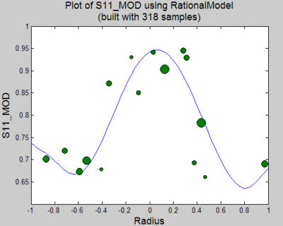
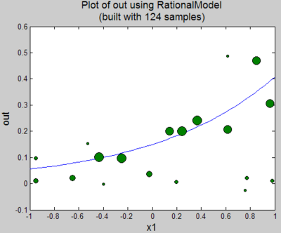
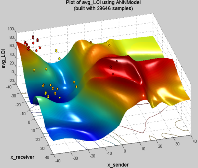
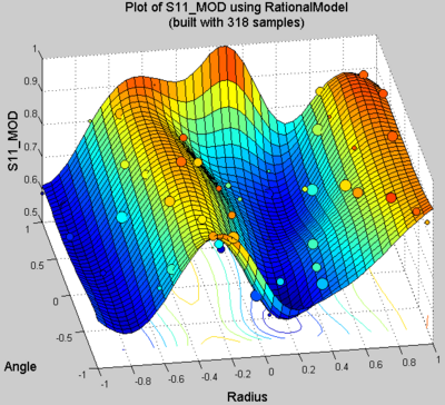
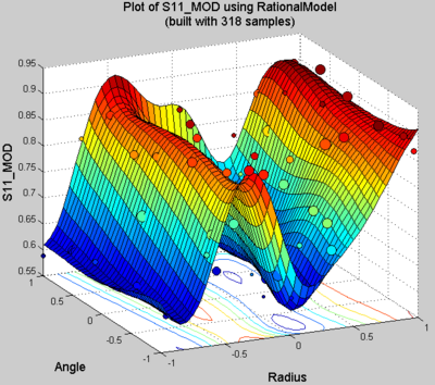
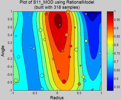
On the right, you can take a look at screenshots of some plots created using the Model Visualization GUI. All plot types are presented. Click on an images to enlarge it.

Getting started

If you want to work with a model saved on disk, you can start the Visualization Console by entering the command guiPlotModel at the Matlab command line. If the command is not found, verify that you have added the toolbox to your path with its startup command. The load from file dialog will appear. After selecting a *.mat file, the model it contains will be loaded and the visualization controls will present themselves. Take a look at the command line options for other ways to start the GUI, or run help guiPlotModel to get an explanation of the options at command line.

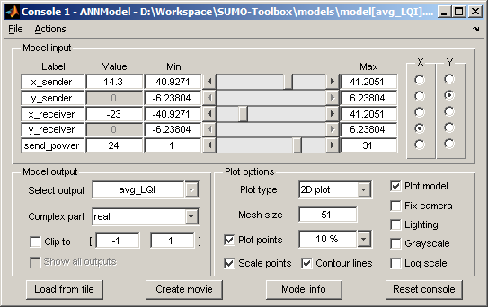
The screenshot below shows a console for a model with five input dimensions on a Windows platform.

Every edit box can be reset to its default value by leaving it empty instead of entering a new value. You can enter any valid Matlab expression in the value and boundary fields, like pi, 5/12 or even 2^(pi*2-4/3).

Model input controls

Every input dimension can be controlled with a single line of the input controls, as shown in the screenshot below.

1. Label: the name of the input parameter, shown as a label on the axis representing it in the plot window;
2. Current value: slice value used when the input is not plotted;
3. Minimum value: lower bound for the axis representing the input;
4. Slider: can be used to change the current value when the input is not plotted;
5. Maximum value: upper bound for the axis representing the input;
6. X radio button: select this radio button to plot the input on the X-axis of the plot;
7. Y radio button: select this radio button to plot the input on the Y-axis of the plot.

It is impossible to show a single input dimension on both X-axis and Y-axis. One input can only be shown on one axis. This constraint is enforced by the GUI. For example, when you click the X radio button of the input that is currently shown on the Y-axis, the new Y-axis will become the topmost free input.

When using the edit fields, keep in mind that the lower bound (minimum) of an input must always be smaller than the upper bound (maximum). The GUI enforces this by adjusting the other boundary when you enter a value that breaks the said constraint. The current value always lies between the boundaries and is adjusted automatically. When an input's upper bound equals its lower bound, you won't be able to change the value and the slider will disappear to indicate this.

Model output controls

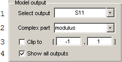
This subsection explains how you can control the model's outputs. The screenshot below shows the part of the console that allows you to do this.

1. Select which output to plot or edit the label of the selected output.
2. Select how to handle complex outputs. You can choose what part of complex numbers must be plotted. Possible choices are to plot only the real part, imaginary part, modulus or angle. The angle is bounded in ]-pi,pi].
3. Clip the output axis. Set the bounds for the output axis to your liking in the edit fields and enable clipping with the Clip to checkbox. The lower bound must always be smaller than the upper bound. If you violate this constraint, the other boundary will be automatically changed so the distance between them is exactly 1. Of course, you can still specify a smaller range manually.
4. When you check this box, all the model's outputs will be shown at the same time, in separate plot windows. All changes made in the console will be applied simultaneously to all plots. You can still switch between outputs, but only to change their labels.

Plot customization controls

These options provide a way to change the visual appearance of the plot.

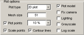
• Different plot types are available: choose between a 1D plot (showing only one input), a 2D plot (showing 2 inputs on a 3D surface) or a Contour plot (showing 2 inputs on a 2D surface, with the output value represented by colour).
• You can set the size of the evaluation grid, used for plotting the model, in the Mesh size field. If plotting is slow, you can try lowering the mesh size to allow for a less accurate but faster visualization.
• A model is built using training samples. These samples are shown in the plot when the Plot points checkbox is enabled. If all dimensions are visible, all points are plotted. However, if not all input dimensions are shown in the plot window, not all samples are plotted. Most of the samples don't have the same fixed slice values as specified with the input controls. Therefore, their output value will most likely be completely different from the output value of the model. Showing all samples would distort the plot and make it impossible to see how far the model really deviates from its samples. Instead, the training samples are filtered according to their distance from the current slice. You can set the maximum distance of points to be plotted, by entering a maximum deviation percentage in the popup/edit box, or selecting a predefined percentage from the list. The deviation percentage is relative to the size of the interval between the minimum and maximum defined for each hidden input dimension. For example, assume we are looking at a model with a single hidden input dimension. Also assume that the maximum deviation is 10 %, the size of the interval is 2 and the current value is val. In this case, all samples with a value inside [val-0.2,val+0.2] will be plotted.
• When not all dimensions are shown in the plot window, the size of the plotted sample points can be set to reflect their distance from the current slice with the Scale points checkbox. The closer the point is to the slice values of the hidden dimensions, the larger it will be shown. Scaling is done linearly between the exact slice value and the maximum deviation specified. If you disable scaling, all visible points will be plotted in the same size.
• In 2D plot mode, you can show the edges of a contour plot below the surface plot by checking the Countour lines checkbox.
• The Plot model checkbox can be disabled if you only want to plot the samples.
• A Fix camera checkbox is provided to keep the camera at a fixed position in successive plots. By default, Matlab always returns the camera to its default position when a figure is plotted. When you enable this option, you override that default behaviour. Fixing the camera is a very important feature if you're exploring a specific part of the plotted figure, or if you simply want to look at the model from a custom position. The camera will always return to its default position when you change the plot type, regardless of the Fix camera setting.
• You can add lighting to the scene in 2D plot mode. Checking the Lighting option adds a light to the scene, in a default position. While the option is enabled, you can add, delete or modify lights in the plot window using the standard Matlab plot edit tools. The modifications will be retained in successive plots.
• By default, all plots use the jet colormap, which varies from dark blue to dark red. You can also use a grayscale colormap, e.g. if you want to print a screenshot with a black and white printer.
• Finally, a checkbox is provided to set a logarithmic scale for the output axis.

Actions

All actions can be accessed from the menu bar, in either the File menu or the Actions menu. Four of those actions are also available via buttons at the bottom of the console.

Through the File menu you can load a model from file by choosing Open. The load from file dialog will open in the directory containing the current model, if it exists. The Reload item allows you to reload the current model from disk. Reloading is especially useful when you are viewing the current best model during a toolbox simulator run. Finally, you can also close the console through this menu.

All other menu items can be found in the Actions menu. A listing of the available actions:

• Open the Create Movie GUI for the current model, so all plot customizations are also applied in the movie.
• Open the Model Info GUI's for the current model.
• Quickly start an optimization of the current model in Matlab's optimization toolbox.
• Take a look at the distribution of training samples across the input dimensions. The sample distribution window shows a scatter plot of the training sample distribution for each pair of input dimensions and box plots for every input dimension separately.
• View a Slice Plot of the current model, retaining all compatible customizations. Most importantly, bounds, labels and lighting options are taken from the console. This Slice Plot can be useful for getting an overall idea of what the model looks like. The number of slices shown can be changed through the command line options.
• Reset all controls to their default values.

The menu items have Alt+<Letter> keyboard shortcuts that can be used while navigating through the menus. Press the Alt key to underline the different letters that can be used as shortcuts. Some actions also have Ctrl+<Letter> keyboard shortcuts, also shown in the menus. The Ctrl shortcuts can be used without having to open the menu.

Title bar

The title bar shows the handles of figures associated with the console and the model type. If the model was loaded from disk, the file name will also be visible in the title bar.

Plot window

The plot window can be edited like any other Matlab plot window. However, you will lose most of your changes once the model plot is refreshed by the console. The changes that can be remembered are the camera settings, light settings and plot title.

Camera and light settings will only be remembered if the corresponding option is checked in the console's plot customization controls. Regardless of those options, camera and light settings will be lost if you change the plot type.

The plot title will be remembered as long as you don't reload the model from disk, rename the plotted output or change the handling of complex outputs. If you want to return to the default title without using one of those options, you can enter __auto__ in the plot title and change any option in the console that refreshes the plot window.

Command line options

Instead of relying on the automatically generated defaults, you can use command line parameters to specify your own settings. The settings passed at command line will be taken as defaults. They are restored when you reset the console. guiPlotModel has the following (optional) parameters:

1. The first parameter is the model to be plotted in the figure window. If you already loaded the model in memory, or simply don't have it saved on disk, you can pass it as a parameter. This disables the reload function, unless you also specify a modelFilename field in the options structure. The field should contain the path to the model on disk.
2. The second parameter represents the index of the output to plot.
3. The third parameter is a structure containing input settings: bounds and values for each input and indices of the inputs to plot. The defaults can be retrieved using settings = defaultInputSettings(model).
4. A structure containing the plot customization options can be passed as the fourth parameter. Get the default options using [dummy options] = guiPlotModel. You don't have to specify all fields when using this parameter. Fields that you don't provide will be set to their default value. With these fields you can specify some additional settings that can't be changed through the GUI:
   • The slices field specifies the number of slices shown in a Slice Plot.
   • The postFunction field can hold a function handle that must be called after each plot. The function should have 1 parameter: the handle to the plot figure. This enables you to easily add an overlay to the plot.
   • You can turn on elevation labels on contour plots by settings the elevationLabels field to true.

Automatically reusing an existing console

A model is equal to another model if it has the same number of inputs and outputs, and all input and output labels are the same. When you try to open the Visualization Console with a model that is equal to a model already shown in a console, the existing console shall be reused. The new model will be inserted in the existing console. The passed settings will be set as the console defaults, but the current settings will not be changed. This is quite useful if you want to look at different instantiations of the same model without having to redo the plot customizations.

Creating a movie

The Create Movie GUI allows you to bring your model to life by varying over (a part of) the domain of a single input parameter. That way, you get an overview of its influence on the model's output. You can create a smooth movie by generating many slices and setting a high frame rate. With a lower frame rate you can create a more explicit succession of slices.

Examples

Here you can take a look at some movies created with the Create Movie GUI. The first and last ones are compressed with Matlab's default AVI codec on Windows, Indeo5. The other examples are presented as QuickTime movies.

• The first movie shows a surface plot that uses lighting and does not show any sample points. The movie has a high framerate and slice count to ensure a smooth transition between frames.
• The second movie illustrates the effect of scaling and filtering sample points in a plot that shows only 1 input dimension. You can see the sample points appear, enlarge, shrink and disappear again as the slice value changes. The largest sample points are the closest to the current slice.
• The third movie is again a surface plot, but now without lighting and a lower framerate. It also shows sample points as seen in the second example.
• The last movie shows a contour plot with scaled and filtered sample points.

Getting started

You can access the Create Movie GUI from the Visualization Console, using the Create movie button at the bottom or in the Actions menu. All customizations applied in the console will be used for the movie. The Create Movie GUI can also be accessed from command line. You won't be able to use any other Matlab GUI component while using the Create Movie GUI. E.g. if you want to further customize the plot with the Visualization Console, press cancel in the Create Movie GUI to return to it.

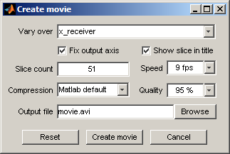
The screenshot of the Create Movie GUI shown below, gives an overview of the available options.

Movie controls

• You can select which input to vary over time with the topmost popup box. All inputs that are not set to be plotted are available. The slices (frames) will be generated over the entire range of the selected input, as specified in the Visualization Console, command line input settings or model defaults. The first slice will have the value of the lower bound; the last one's value will be equal to the upper bound.
• On the second line you can see two checkboxes. The first one specifies if the output axis should be clipped to the maximum and minimum output values found in all slices. Keep this checkbox selected if you want to prevent that the axis scale changes during the movie, which causes irregular jumps in the successive plots. However, enabling this option also means creating the movie will take longer, because the correct clipping bounds can only be known after all slices have been generated. The slices will be reloaded from disk and modified to the custom bounds. To avoid this second pass and prevent the output axis scale from changing during the movie, you can enable output clipping in advance. Using the Visualization Console, you can explore the model to get an idea of a good set of bounds to use. Enable the 'Clip to checkbox found at the bottom left of the Visualization Console to clip the output.
• By default, the title of each slice plot in the movie shows the current slice value of the input varying over time. This option can be toggled with the Show slice in title checkbox.
• Specify how many slices should be generated in the Slice count field.
• To the right of the slices field you can enter the number of frames per second to be shown in the movie. Fractions can be used. For example, 0.2 fps means each slice will be shown for five seconds. You can enter a number yourself or select one from the popup box.
• Movies are created using the default Matlab codec by default. On Linux platforms, this is an uncompressed AVI format. On other platforms, the default Matlab codec does support compression. When compression is supported, the compression quality can be set using the popup/edit box to the right of the compression popup box. If you have the Java Media Framework installed and in Matlab's Java class path, you can also create QuickTime movies, but that codec does not allow you to specify a compression quality.
• The Output file field shows the path to the file where the movie shall be created. You can enter a file path manually or use the browse button. The correct file extension for the selected codec is automatically appended to the file path.
• At the bottom of the window there are 3 buttons. The button on the left resets all fields in the window to their default value. The button on the right closes the window. The middle button starts the movie generation process. During the generation process, the plot window will be made visible above all other Matlab windows. Some progress information will be printed at the Matlab command line.
• Upon pressing the Create movie button, the current settings (except for the selected input dimension) are stored in memory, for the duration of your current Matlab session. The next time you open the Create Movie GUI, the saved settings will be restored. This is a handy feature if you want to create several movies using the same settings.

Command line options

Instead of starting the Create Movie GUI through the Visualization Console, you can also start it directly from command line using the Matlab command guiCreateMovie. Without parameters, a load from file dialog will appear so you can select a model stored on disk. Below are the optional parameters to the command, in order of appearance.

1. The first parameter is the model to be plotted in the figure window. If you already loaded the model in memory, or simply don't have it saved on disk, you can pass it as a parameter.
2. The second parameter represents the index of the output to plot.
3. The third parameter is a structure containing input settings: bounds and values for each input and indices of the inputs to plot. The defaults can be retrieved using settings = defaultInputSettings(model).
4. A structure containing the plot customization options can be passed as the fourth parameter. Retrieve the defaults using [dummy1 dummy2 options] = quickPlotModel. You don't have to specify all fields when using this parameter. Fields that you don't provide will be set to their default value.
5. If you want to plot the slices of the movie in a specific figure window, pass its handle as the fifth parameter. Otherwise the current figure will be used.

The first four parameters are in the same order as used to start the Visualization Console from command line. As with the Visualization Console, the command help guiCreateMovie will provide a brief description of the function and its parameters, in the correct order.

Reusing the generated slices

Next to the actual movie file, a subdirectory slices shall be created containing all slices used in the movie, in png format. If you enabled the Fix output axis option, you will also find a Matlab figure file for every slice in that directory. The Fix output axis option is only applied to the png files. The slices subdirectory will be erased when starting a new movie generation process in the same directory.

You might want to create several movies from the same slices, but with different output formats or frame rates. This process can be speeded up by using the Matlab command images2movie. It allows you to create a movie from an existing directory of images. These are the parameters to the function:

1. path to the directory containing the images;
2. file path to the location where the movie should be saved (the file extension defines the video codec);
3. file extension of the images, in this case png;
4. number of frames per second;
5. compression quality percentage.

Creating a movie from command line

Instead of creating a movie using the GUI, you can use the genMovie command to create one from command line. The parameters to the command are the same as the parameters to the Create Movie GUI with the addition of a sixth optional parameter containing the movie options. The default movie options can be retrieved with the command options = genMovie. Like elsewhere, the options structures don't have to be complete. Fields that you don't provide will be set to their default value. You can run help genMovie for more information at command line.

Since the command doesn't use a GUI, the first parameter is no longer optional if you want to create a movie. You have to pass a model already present in the Matlab workspace as the first parameter. See #Loading a model from disk for an easy way to load a model into the Matlab workspace.

Viewing model information

The Model Information GUI gives you a quick overview of a model. It shows any model's error statistics, scores, description, dimensions and more. Some information fields are specific to the selected output; others are specific to the model only. You can select which output's information you want to see. Additionally, you can specify an external validation set or function to compute error statistics. You can compare your customized statistics to the training error statistics.

All information fields contain selectable text, so you can easily copy the information you want to the clipboard.

Getting started

The Model Information GUI can quickly be started from the Visualization Console, by clicking the button at the bottom of the console or through the Actions menu. It can also be accessed from Matlab's command line.

Controls

The controls, visible in the screenshot below, are positioned in the top right corner of the Model Information GUI.

• You can select which output's error statistics, error plots and expression must be shown using a popup box.
• External validation data can be selected from another popup box. All matrices of doubles and function handles in the workspace are listed. You must select a valid matrix or function handle. If the selected workspace variable is invalid, an error message will be shown in a dialog box and external validation will be deactivated. You can deactivate external validation by selecting the empty matrix [] from the popup box. Validation data provided at command line is listed as command line. See #Using external validation data for more information.
• When using a function handle for external validation, an evaluation grid will be constructed for you. The maximum number of points to use for constructing the evaluation grid can be specified. The points will be linearly spaced along the model's input dimension ranges.
• Finally, a checkbox allows you to use logarithmic scaling for the Y axis in the error plots.

Using external validation data

External validation can be computed in two ways. You can provide a complete dataset of expected values or a handle of a function that computes these expected values. The dataset must be a matrix with a column for every input and output, in the correct order. The first columns must represent the input values; the last columns must represent the corresponding output values. The function handle must take an evaluation grid as its single input parameter and return a matrix with a column for each of the model's outputs. The return matrix must specify the expected output values corresponding to the input values specified in the input matrix.

The validation matrix or function should be present as a variable in the Matlab workspace, ideally before starting the Model Information GUI. If you want to use a variable added to the workspace after you started the GUI, you first have to reset the GUI using Ctrl+R or by clicking Reset in the Actions menu.

Actions

In addition to the controls available in the top right corner of the GUI, some actions are available through the menu. The File menu enables you to open another model in the current Model Information GUI, reload the current model or close the GUI window. Through the Actions menu, you can reset the GUI controls and fields to their default values. That menu also allows you to export the model to a Matlab M-file for using it outside the SUMO Toolbox.

Like in the Visualization Console, the menu items have Alt+<Letter> keyboard shortcuts that can be used while navigating through the menus. Press the Alt key to underline the different letters that can be used as shortcuts. Some actions also have Ctrl+<Letter> keyboard shortcuts, which are also shown in the menus. The Ctrl shortcuts can be accessed without having to open the menu.

Error plots

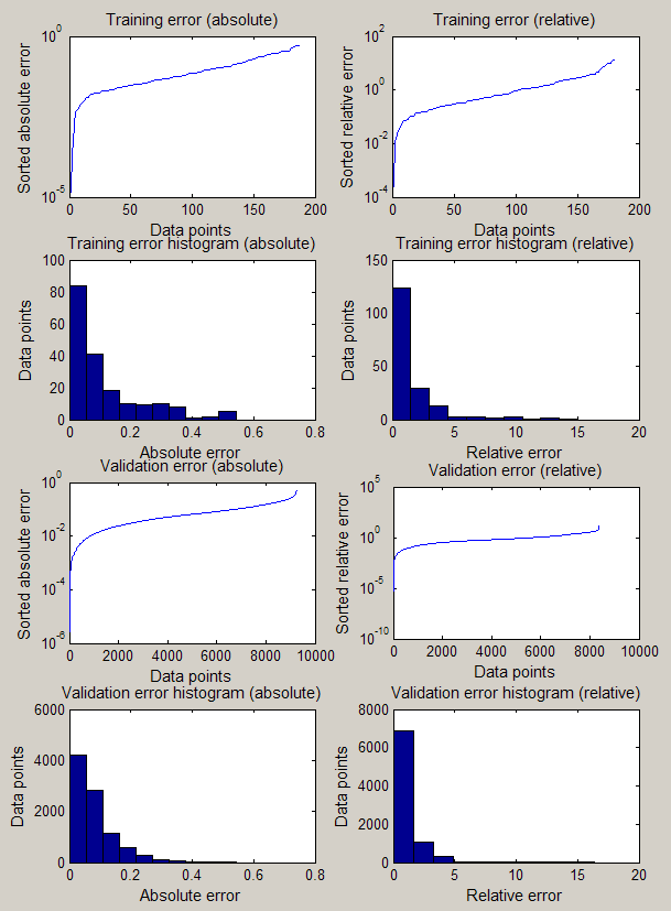
On the left side of the Model Information GUI, plots representing the error statistics for the currently selected output are presented. The top four plots represent the errors in the training samples. If you specify valid external validation data, another four plots will be shown, representing the errors computed with that validation data.

This screenshot shows error plots for both training samples and using an external validation matrix.

Both absolute and relative errors are shown. The plots on the left show the absolute error, the plots on the right show the relative error. Two plot types are used for showing the errors. The upper plot shows the validation error against the number of points that remain below it. The lower plot is a histogram that groups the points by their error. The relative error histograms don't include any samples with an infinite relative error, because they would cripple the entire histogram and render it useless.

Information fields

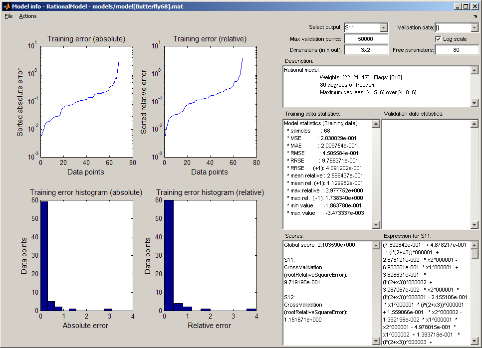
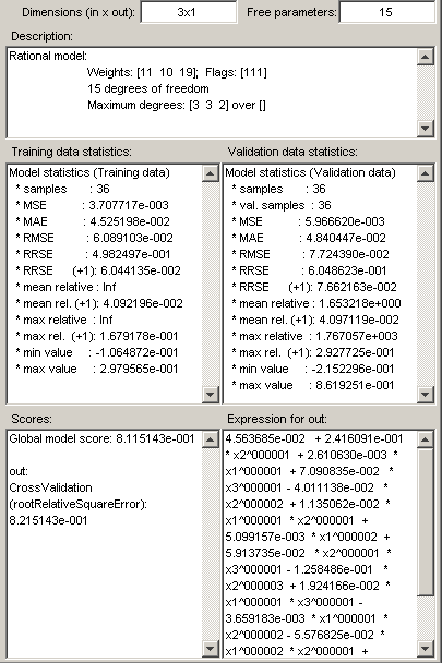
All information fields are presented on the right hand side of the GUI, below the controls. Here you can look at a screenshot of those fields alone.

• At the top left of the screenshot you can see a field specifying the number of inputs and outputs of the current model. Next to it stands the number of free parameters used for constructing the model.

• A general model description is presented in the Description field.

• The middle fields contain error statistics for the current output. On the left the statistics measured against the training data are shown. The field on the right shows statistics for the external validation set or function you specified. If no external validation data is set, this field will be empty.

• The field at the bottom left shows the scores computed while generating the model. Both a global score and a list of scores for every output are provided. To the right of the scores field you can see the expression used inside the model for computing the value of the current output. This expression can become quite large for difficult models, so you will have to use the scroll bar attached to the field for seeing it completely.

Title bar

The title bar shows the type of model currently shown in the GUI. If the model was loaded from disk, the file name will also be visible in the title bar.

Command line options

Instead of starting the Model Information GUI through the Visualization Console, you can also start it directly from command line using the Matlab command guiModelInfo. Without parameters, a load from file dialog will appear so you can select a model stored on disk. Below are the parameters to the command, in order of appearance. All parameters are optional, except the first one.

1. The model whose information you want to view must be provided as the first parameter. If you already loaded the model in memory, or simply don't have it saved on disk, you can provide it here.
2. The second parameter is the index of the output for which output specific information must be shown.
3. You can pass validation data directly as the third command line parameter. You can always return to the validation data specified at command line by selecting command line in the validation popup box. See #Using external validation data for more information.
4. Specify the path to the mat file containing the model as the fourth parameter. Doing so will enable you to reload it from disk, even when you passed it at command line. Leave this parameter empty if you don't have a file containing the model.
5. The last parameter is a small options structure. The defaults can be retrieved using [dummy options] = guiPlotModelErrors. You don't have to specify all fields when using this parameter. Fields that you don't provide will be set to their default value.

The first two parameters are in the same order as used to start the Visualization Console from command line. The command help guiModelInfo will provide a brief description of the function and its parameters, in the correct order.

Loading a model from disk

The GUI comes with an easy to use command for loading a model from disk into the Matlab workspace: guiLoadModel. It provides the load from file dialogs for the three GUI components explained above, but you can also use it separately. You can specify a starting path for the dialog as an optional parameter. The function returns the loaded model as the first return parameter, and the name of the file containing the model as the second return parameter. Run help guiLoadModel to get a short description of the function and its parameters at command line.