Difference between revisions of "About"
| (160 intermediate revisions by 9 users not shown) | |||
| Line 1: | Line 1: | ||
== History == | == History == | ||
| − | In 2004, research within the COMS group was focused on developing efficient, adaptive and accurate algorithms for polynomial and rational modeling of linear time-invariant (LTI) systems. This work resulted in a set of Matlab scripts that were used as a testing ground for new ideas and | + | In 2004, research within the (former) COMS research group, led by professor [http://www.sumo.intec.ugent.be/?q=tomd Tom Dhaene], was focused on developing efficient, adaptive and accurate algorithms for polynomial and rational modeling of linear time-invariant (LTI) systems. This work resulted in a set of Matlab scripts that were used as a testing ground for new ideas and concepts. Research progressed, and with time these scripts were re-worked and refactored into one coherent Matlab toolbox, tentatively named the Multivariate MetaModeling (M3) Toolbox. The first public release of the toolbox (v2.0) occurred in November 2006. In October 2007, the development of the M3 Toolbox was discontinued. |
| − | == | + | [[Image:Sumo.jpg|150 px|right|blindDACE Toolbox]] |
| + | In April 2008, the first public release of the Surrogate Modeling (SUMO) Toolbox (v5.0) occurred. | ||
| + | |||
| + | For a list of changes since then refer to the [[Changelog]] and [[Whats new]] pages. | ||
| + | |||
| + | == Intended use == | ||
=== Global Surrogate Models === | === Global Surrogate Models === | ||
| − | The | + | The SUMO Toolbox was originally designed to solve the following problem: |
| − | <center>'' | + | <center>''Automatically generate a highly accurate surrogate model (= a regression model) for a computational expensive simulation code |
| + | <br>requiring as little data points and as little user-interaction as possible.''</center> | ||
In addition the toolbox provides powerful, adaptive algorithms and a whole suite of model types for | In addition the toolbox provides powerful, adaptive algorithms and a whole suite of model types for | ||
| − | * data fitting problems (regression) | + | * data fitting problems (regression, function approximation, curve fitting) |
| − | * response surface modeling | + | * response surface modeling (RSM) |
| − | * interpolation | + | * scattered data interpolation |
| − | * optimal | + | * model selection |
| + | * Design Of Experiments (DoE) | ||
| + | * model parameter optimization, e.g., finding the optimal neural network topology, SVM kernel parameters, rational function order, etc. (= hyperparameter optimization) | ||
| + | * iterative adaptive sample selection (also known as sequential design or active learning) | ||
| + | |||
| + | Note that the SUMO toolbox is able to drive the simulation code directly. | ||
| − | For | + | For domain experts or engineers the SUMO Toolbox provides a flexible, pluggable platform to which the response surface modeling task can be delegated. For researchers in surrogate modeling it provides a common framework to implement, test and benchmark new modeling and sampling algorithms. |
| − | See the Wikipedia [http://en.wikipedia.org/wiki/Surrogate_model | + | See the Wikipedia [http://en.wikipedia.org/wiki/Surrogate_model surrogate model] page to find out more. |
=== Surrogate Driven Optimization === | === Surrogate Driven Optimization === | ||
| − | While the main focus of the | + | While the main focus of the SUMO Toolbox is to create accurate global surrogate models, it can be used for other goals too. |
| + | |||
| + | For instance, the toolbox can be used to create consecutive local surrogate models for optimization purposes. The information obtained from the local surrogate models is used to guide the adaptive sampling process to the global optimum. | ||
| + | |||
| + | A good sample strategy for surrogate driven optimization seeks a balance between local search and global search, or refining the surrogate model and finding the optimum. | ||
| + | Such a sample strategy is implemented (akin to (Super)EGO), see the different [[Sample_Selectors#expectedImprovement|sample selectors]] for more information. | ||
| + | |||
| + | === Dynamic systems or Time series prediction === | ||
| + | |||
| + | See [[FAQ#What_about_dynamical.2C_time_dependent_data.3F]]. | ||
| + | |||
| + | === Classification === | ||
| + | |||
| + | See [[FAQ#What_about_classification_problems.3F]]. | ||
| + | |||
| + | == Application range == | ||
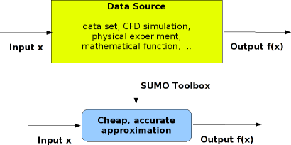
| + | The SUMO Toolbox has already been applied successfully to a wide range of problems from domains as diverse as aerodynamics, geology, metallurgy, electro-magnetics (EM), electronics, engineering and economics. The SUMO Toolbox can be applied to any situation where the problem can be described as a function that maps a set of inputs onto a set of outputs. We generally refer to this function as the [[Simulator]]. | ||
| + | |||
| + | |||
| + | [[Image:sumotask.png|center|SUMO-Toolbox : Generating an approximation for a reference model]] | ||
| + | |||
| + | Across the different problems to which we have applied the toolbox, the input dimension has ranged from 1 to 130 and the output dimension from 1 to 70 (including both complex and real valued outputs). The number of data points has ranged from as little as 15 to as many as 100000. | ||
| + | |||
| + | == Design goals == | ||
| + | |||
| + | The SUMO Toolbox was designed with a number of goals in mind: | ||
| − | + | * A flexible tool that integrates different modeling methods and does not tie the user down to one particular set of problems. Reliance on domain specific features should be avoided. | |
| − | + | * The focus should be on adaptivity, i.e., relieving the burden on the domain expert as much as possible. Given a simulation model, the software should produce an accurate surrogate model with minimal user interaction. This also includes easily integrating with the existing design environment. | |
| − | |||
| − | + | * At the same time keeping in mind that there is no such thing as a `one-size-fits-all'. Different problems need to be modeled differently and require different a priori process knowledge. Therefore the software should be modular and easily extensible to new methods. | |
| − | |||
| − | |||
| − | |||
| − | |||
| − | + | * Engineers or domain experts do not tend to trust a black box system that generates models but is unclear about the reasons why a particular model should be preferred. Therefore an important design goal was that the expert user should be able to have full manual control over the modeling process if necessary. In addition the toolbox should support fine grain logging and profiling capabilities so its modeling and sampling decisions can be retraced. | |
| − | + | Given this design philosophy, the toolbox can cater to both the researchers working on novel surrogate modeling techniques as well as to the engineers who need the surrogate model as part of their design process. For the former, the toolbox provides a common platform on which to deploy, test, and compare new modeling algorithms and sampling techniques. For the latter, the software functions as a highly configurable and flexible component to which surrogate model construction can be delegated, easing the burden of the user and enhancing productivity. | |
| − | |||
| − | |||
| − | |||
| − | |||
== Features == | == Features == | ||
| − | The main features of the toolbox | + | The main features of the toolbox are listed below. For an overview of recent changes see the [[Whats new]] page. A detailed list of changes can be found in the [[Changelog]]. |
{| class="wikitable" style="text-align:left" border="0" cellpadding="5" cellspacing="0" | {| class="wikitable" style="text-align:left" border="0" cellpadding="5" cellspacing="0" | ||
| − | ! | + | ! Implementation Language |
| − | | | + | | Matlab, Java, and where applicable C, C++ |
|- | |- | ||
| − | ! | + | ! Design patterns |
| − | | | + | | Fully object oriented, with the focus on clean design and encapsulation. |
|- | |- | ||
! Minimum Requirements | ! Minimum Requirements | ||
| − | | | + | | See the [[system requirements]] page |
|- | |- | ||
! Supported data sources* | ! Supported data sources* | ||
| − | | Local executable/script, | + | | Local executable/script, simulation engine, Java class, Matlab script, dataset (txt file) (see [[Interfacing with the toolbox]]) |
|- | |- | ||
! Supported data types | ! Supported data types | ||
| Supports multi-dimensional inputs and outputs. Outputs can be any combination of real/complex. | | Supports multi-dimensional inputs and outputs. Outputs can be any combination of real/complex. | ||
| + | |- | ||
| + | ! Supported problem types | ||
| + | | Regression ([[FAQ#What_about_classification_problems.3F|classification]], [[FAQ#What_about_dynamical.2C_time_dependent_data.3F|time series prediction]]) | ||
|- | |- | ||
! Configuration | ! Configuration | ||
| − | | Extensively configurable through one main XML configuration file. | + | | Extensively configurable through one main [[FAQ#What_is_XML.3F|XML]] configuration file. |
|- | |- | ||
! Flexibility | ! Flexibility | ||
| Line 67: | Line 97: | ||
|- | |- | ||
! Predefined accuracy | ! Predefined accuracy | ||
| − | | The toolbox will run until the user required accuracy has been reached | + | | The toolbox will run until the user required accuracy has been reached, the maximum number of samples has been exceeded or a timeout has occurred |
|- | |- | ||
! Model Types* | ! Model Types* | ||
| Out of the box support for: | | Out of the box support for: | ||
| − | + | * Polynomial/Rational functions | |
| − | + | * Feedforward Neural Networks, 3 implementations | |
| − | + | ** One based on the [http://www.mathworks.com/products/neuralnet/ Matlab Neural Network toolbox] | |
| − | + | ** One based on the [http://leenissen.dk/fann/ Fast Artificial Neural Network Library (FANN)] | |
| − | + | ** One based on the [http://www.iau.dtu.dk/research/control/nnsysid.html NNSYSID Toolbox] | |
| − | + | ** One based on Extreme Learning Machine (ELM) | |
| − | + | * Radial Basis Function (RBF) Models | |
| − | + | * RBF Neural Networks | |
| − | + | * Gaussian Process Models (based on [http://www.GaussianProcess.org/gpml/code GPML]) | |
| − | + | * Kriging Models (two custom implementations) | |
| + | * Blind Kriging Models | ||
| + | * Smoothing spline models | ||
| + | * Support Vector Machines (SVM) | ||
| + | ** Least Squares SVM (based on [http://www.esat.kuleuven.ac.be/sista/lssvmlab/ LS-SVMlab]) | ||
| + | ** epsilon-SVM (based on [http://www.csie.ntu.edu.tw/~cjlin/libsvm/ LIBSVM] or [http://svmlight.joachims.org/ SVMlight]) | ||
| + | ** nu-SVM (based on [http://www.csie.ntu.edu.tw/~cjlin/libsvm/ LIBSVM]) | ||
| + | * Support for model types from the [http://www.cs.waikato.ac.nz/ml/weka/ WEKA] data mining library | ||
| + | ** Classification, regression and clustering algorithms present in WEKA can be used simply by adding entries in the configuration. Please refer to the 'weka' ModelBuilder in the demo configuration file. A list of algorithms can be found [http://wiki.pentaho.com/display/DATAMINING/Data+Mining+Algorithms+and+Tools+in+Weka here]. | ||
|- | |- | ||
| − | ! | + | ! Model parameter optimization algorithms* |
| − | | Pattern Search, Simulated Annealing, Genetic Algorithm, BGFS, ... | + | | Pattern Search, EOG, Simulated Annealing, Genetic Algorithm, BGFS, DIRECT, Particle Swarm Optimization (PSO), NSGA-II ... |
|- | |- | ||
| − | ! | + | ! Sample selection algorithms (=sequential design, active learning)* |
| − | | Random, error based, density based, gradient based | + | | Random, error-based, density-based, gradient-based, and many different hybrids |
|- | |- | ||
! Experimental design* | ! Experimental design* | ||
| − | | Latin Hypercube Sampling, Central Composite, random, | + | | Latin Hypercube Sampling, Central Composite, Box-Behnken, random, user defined, full factorial |
|- | |- | ||
! Model selection measures* | ! Model selection measures* | ||
| − | | Validation set, cross-validation, | + | | Validation set, cross-validation, leave-one-out, model difference, AIC (also in a multi-objective context, see [[Multi-Objective Modeling]]), LRM |
|- | |- | ||
! Sample Evaluation* | ! Sample Evaluation* | ||
| Line 98: | Line 136: | ||
|- | |- | ||
! Supported distributed middlewares* | ! Supported distributed middlewares* | ||
| − | | [http://gridengine.sunsource.net/ Sun Grid Engine], LCG Grid middleware (both accessed through a SSH accessible frontnode | + | | [http://gridengine.sunsource.net/ Sun Grid Engine], LCG Grid middleware (both accessed through a SSH accessible frontnode) |
|- | |- | ||
! Logging | ! Logging | ||
| − | | Extensive | + | | Extensive logging to enable close monitoring of the modeling process. Logging granularity is fully configurable and log streams can be easily redirected (to file, console, a remote machine, ...). |
|- | |- | ||
! Profiling* | ! Profiling* | ||
| − | | Extensive profiling framework for easy gathering (and plotting) of modeling metrics | + | | Extensive profiling framework for easy gathering (and plotting) of modeling metrics (average sample evaluation time, hyperparameter optimization trace, ...) |
|- | |- | ||
! Easy tracking of modeling progress | ! Easy tracking of modeling progress | ||
| Automatic storing of best models and their plots. Ability to automatically generate a movie of the sequence of plots. | | Automatic storing of best models and their plots. Ability to automatically generate a movie of the sequence of plots. | ||
| + | |- | ||
| + | ! Model browser GUI | ||
| + | | A graphical tool is available to easily visualize high dimensional models and browse through data ([[Model Visualization GUI|more information here]]) | ||
|- | |- | ||
! Available test problems* | ! Available test problems* | ||
| − | | Out of the box support for | + | | Out of the box support for many built-in functions (Ackley, Camel Back, Goldstein-Price, ...) and datasets (Abalone, Boston Housing, FishLength, ...) from various application domains. Including a number of datasets (and some simulation code) from electronics. In total over 50 examples are available. |
| + | |- | ||
| + | ! License | ||
| + | | [[License terms]] | ||
|} | |} | ||
| Line 116: | Line 160: | ||
== Screenshots == | == Screenshots == | ||
| − | A number of screenshots to give | + | A number of screenshots to give a feel of the SUMO Toolbox. Note these screenshots do not necessarily reflect the latest toolbox version. |
<gallery> | <gallery> | ||
| − | Image: | + | Image:octagon.png |
| − | Image: | + | Image:metamodel-sumo-hourglass.png |
| − | Image: | + | Image:SUMO_Toolbox1.png |
| + | Image:SUMO_Toolbox2.png | ||
| + | Image:SUMO_Toolbox3.png | ||
| + | Image:SUMO_Toolbox4.png | ||
| + | Image:ISCSampleSelector1.png | ||
| + | Image:ISCSampleSelector2.png | ||
| + | Image:SUMO_Gui1.png | ||
| + | Image:SUMO_Gui2.png | ||
| + | Image:Contour1.png | ||
| + | Image:TwoDim1.png | ||
| + | Image:TwoDim2.png | ||
| + | Image:ThreeDim1.png | ||
| + | Image:ThreeDim2.png | ||
| + | Image:ThreeDim3.png | ||
| + | Image:FEBioTrekEI.png | ||
| + | Image:FEBioTrekFunc.png | ||
</gallery> | </gallery> | ||
== Movies == | == Movies == | ||
| − | |||
| − | + | [[Image:youtube-logo.jpg|right|70px|link=http://www.youtube.com/sumolab|]] A number of video clips generated by or related to the SUMO Toolbox [http://www.youtube.com/sumolab can be found at our YouTube channel]. Feel free to make suggestions or leave comments. | |
| − | + | ||
| − | + | Note these movies do not necessarily reflect the latest toolbox version. Improvements and/or interface adjustments may have been made since then. | |
== Documentation == | == Documentation == | ||
| − | + | An in depth overview of the rationale and philosophy, including a treatment of the software architecture underlying the SUMO Toolbox is available in the form of a PhD dissertation. A copy of this dissertation [[Media:2010Gorissen_SUMO.pdf|is available here]]. | |
| − | |||
| − | |||
| − | |||
| − | |||
| − | + | In addition the following poster and presentation give a high level overview: | |
| − | |||
| − | |||
| − | |||
| − | + | * Poster: [[Media:SUMO_poster.pdf|SUMO poster]] | |
| + | * Presentation: [[Media:SUMO_presentation.pdf|SUMO slides]] | ||
| − | + | A blog covering related research can be found here [http://sumolab.blogspot.com http://sumolab.blogspot.com]. | |
| − | == | + | == Citations == |
See [[Citing|Citing the toolbox]]. | See [[Citing|Citing the toolbox]]. | ||
Latest revision as of 10:24, 17 March 2015
History
In 2004, research within the (former) COMS research group, led by professor Tom Dhaene, was focused on developing efficient, adaptive and accurate algorithms for polynomial and rational modeling of linear time-invariant (LTI) systems. This work resulted in a set of Matlab scripts that were used as a testing ground for new ideas and concepts. Research progressed, and with time these scripts were re-worked and refactored into one coherent Matlab toolbox, tentatively named the Multivariate MetaModeling (M3) Toolbox. The first public release of the toolbox (v2.0) occurred in November 2006. In October 2007, the development of the M3 Toolbox was discontinued.
In April 2008, the first public release of the Surrogate Modeling (SUMO) Toolbox (v5.0) occurred.
For a list of changes since then refer to the Changelog and Whats new pages.
Intended use
Global Surrogate Models
The SUMO Toolbox was originally designed to solve the following problem:
requiring as little data points and as little user-interaction as possible.
In addition the toolbox provides powerful, adaptive algorithms and a whole suite of model types for
- data fitting problems (regression, function approximation, curve fitting)
- response surface modeling (RSM)
- scattered data interpolation
- model selection
- Design Of Experiments (DoE)
- model parameter optimization, e.g., finding the optimal neural network topology, SVM kernel parameters, rational function order, etc. (= hyperparameter optimization)
- iterative adaptive sample selection (also known as sequential design or active learning)
Note that the SUMO toolbox is able to drive the simulation code directly.
For domain experts or engineers the SUMO Toolbox provides a flexible, pluggable platform to which the response surface modeling task can be delegated. For researchers in surrogate modeling it provides a common framework to implement, test and benchmark new modeling and sampling algorithms.
See the Wikipedia surrogate model page to find out more.
Surrogate Driven Optimization
While the main focus of the SUMO Toolbox is to create accurate global surrogate models, it can be used for other goals too.
For instance, the toolbox can be used to create consecutive local surrogate models for optimization purposes. The information obtained from the local surrogate models is used to guide the adaptive sampling process to the global optimum.
A good sample strategy for surrogate driven optimization seeks a balance between local search and global search, or refining the surrogate model and finding the optimum. Such a sample strategy is implemented (akin to (Super)EGO), see the different sample selectors for more information.
Dynamic systems or Time series prediction
See FAQ#What_about_dynamical.2C_time_dependent_data.3F.
Classification
See FAQ#What_about_classification_problems.3F.
Application range
The SUMO Toolbox has already been applied successfully to a wide range of problems from domains as diverse as aerodynamics, geology, metallurgy, electro-magnetics (EM), electronics, engineering and economics. The SUMO Toolbox can be applied to any situation where the problem can be described as a function that maps a set of inputs onto a set of outputs. We generally refer to this function as the Simulator.
Across the different problems to which we have applied the toolbox, the input dimension has ranged from 1 to 130 and the output dimension from 1 to 70 (including both complex and real valued outputs). The number of data points has ranged from as little as 15 to as many as 100000.
Design goals
The SUMO Toolbox was designed with a number of goals in mind:
- A flexible tool that integrates different modeling methods and does not tie the user down to one particular set of problems. Reliance on domain specific features should be avoided.
- The focus should be on adaptivity, i.e., relieving the burden on the domain expert as much as possible. Given a simulation model, the software should produce an accurate surrogate model with minimal user interaction. This also includes easily integrating with the existing design environment.
- At the same time keeping in mind that there is no such thing as a `one-size-fits-all'. Different problems need to be modeled differently and require different a priori process knowledge. Therefore the software should be modular and easily extensible to new methods.
- Engineers or domain experts do not tend to trust a black box system that generates models but is unclear about the reasons why a particular model should be preferred. Therefore an important design goal was that the expert user should be able to have full manual control over the modeling process if necessary. In addition the toolbox should support fine grain logging and profiling capabilities so its modeling and sampling decisions can be retraced.
Given this design philosophy, the toolbox can cater to both the researchers working on novel surrogate modeling techniques as well as to the engineers who need the surrogate model as part of their design process. For the former, the toolbox provides a common platform on which to deploy, test, and compare new modeling algorithms and sampling techniques. For the latter, the software functions as a highly configurable and flexible component to which surrogate model construction can be delegated, easing the burden of the user and enhancing productivity.
Features
The main features of the toolbox are listed below. For an overview of recent changes see the Whats new page. A detailed list of changes can be found in the Changelog.
| Implementation Language | Matlab, Java, and where applicable C, C++ |
|---|---|
| Design patterns | Fully object oriented, with the focus on clean design and encapsulation. |
| Minimum Requirements | See the system requirements page |
| Supported data sources* | Local executable/script, simulation engine, Java class, Matlab script, dataset (txt file) (see Interfacing with the toolbox) |
| Supported data types | Supports multi-dimensional inputs and outputs. Outputs can be any combination of real/complex. |
| Supported problem types | Regression (classification, time series prediction) |
| Configuration | Extensively configurable through one main XML configuration file. |
| Flexibility | Virtually every component of the modeling process can be configured, replaced or extended by a user specific, custom implementation |
| Predefined accuracy | The toolbox will run until the user required accuracy has been reached, the maximum number of samples has been exceeded or a timeout has occurred |
| Model Types* | Out of the box support for:
|
| Model parameter optimization algorithms* | Pattern Search, EOG, Simulated Annealing, Genetic Algorithm, BGFS, DIRECT, Particle Swarm Optimization (PSO), NSGA-II ... |
| Sample selection algorithms (=sequential design, active learning)* | Random, error-based, density-based, gradient-based, and many different hybrids |
| Experimental design* | Latin Hypercube Sampling, Central Composite, Box-Behnken, random, user defined, full factorial |
| Model selection measures* | Validation set, cross-validation, leave-one-out, model difference, AIC (also in a multi-objective context, see Multi-Objective Modeling), LRM |
| Sample Evaluation* | On the local machine (taking advantage of multi-core CPUs) or in parallel on a cluster/grid |
| Supported distributed middlewares* | Sun Grid Engine, LCG Grid middleware (both accessed through a SSH accessible frontnode) |
| Logging | Extensive logging to enable close monitoring of the modeling process. Logging granularity is fully configurable and log streams can be easily redirected (to file, console, a remote machine, ...). |
| Profiling* | Extensive profiling framework for easy gathering (and plotting) of modeling metrics (average sample evaluation time, hyperparameter optimization trace, ...) |
| Easy tracking of modeling progress | Automatic storing of best models and their plots. Ability to automatically generate a movie of the sequence of plots. |
| Model browser GUI | A graphical tool is available to easily visualize high dimensional models and browse through data (more information here) |
| Available test problems* | Out of the box support for many built-in functions (Ackley, Camel Back, Goldstein-Price, ...) and datasets (Abalone, Boston Housing, FishLength, ...) from various application domains. Including a number of datasets (and some simulation code) from electronics. In total over 50 examples are available. |
| License | License terms |
* Custom implementations can easily be added
Screenshots
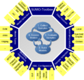
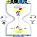
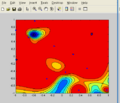
A number of screenshots to give a feel of the SUMO Toolbox. Note these screenshots do not necessarily reflect the latest toolbox version.
Movies
A number of video clips generated by or related to the SUMO Toolbox can be found at our YouTube channel. Feel free to make suggestions or leave comments.
Note these movies do not necessarily reflect the latest toolbox version. Improvements and/or interface adjustments may have been made since then.
Documentation
An in depth overview of the rationale and philosophy, including a treatment of the software architecture underlying the SUMO Toolbox is available in the form of a PhD dissertation. A copy of this dissertation is available here.
In addition the following poster and presentation give a high level overview:
- Poster: SUMO poster
- Presentation: SUMO slides
A blog covering related research can be found here http://sumolab.blogspot.com.
Citations
See Citing the toolbox.
